
1. The Problem: From RAW Acquisition to Diagnostic Quality
The effectiveness of medical image pre-processing determines the accuracy of the entire diagnostic pipeline, but the advent of conventional AI has introduced concrete risks of visual hallucinations.
A digital radiographic image is the result of a complex physical and computational chain. As described in the D/Vision Lab article “Dalla Fisica alla Diagnosi: Come strutturare una Pipeline di Pre-Processing nell’Imaging Medicale”, , the signal originates from subatomic interactions—specifically, the photoelectric effect and Compton scattering—and is converted into a 14- or 16-bit digital matrix via flat-panel detectors. The raw output, typically a 16-bit TIFF file, is rarely ready for clinical interpretation.
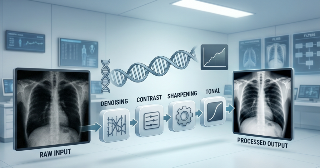
The RAW image carries the signatures of this entire physical chain, necessitating a targeted medical image pre-processing protocol to mitigate electronic and quantum noise, defective pixels, sensor non-uniformity (fixed-pattern noise), beam-hardening artifacts, and dispersion blur. Before it can be interpreted by a radiologist, or an AI algorithm, it must pass through a preprocessing pipeline: a sequence of operations including denoising, sharpening, contrast correction, and tonal adjustment.
The core problem is that there is no universal pipeline. Every modality (X-ray, CT, digital microscopy), every scanner manufacturer, and every clinical protocol produces images with unique noise, contrast, and resolution characteristics. The calibration process is traditionally manual: an expert experiments with combinations of filters, visually evaluates the output, and adjusts parameters, sometimes for days.
The key question: Given a dataset of raw-image / reference-image pairs processed by an expert, is it possible to automatically learn the optimal pipeline? And can we do it in a way that generalizes to new, unseen images during optimization?
The answer is yes, but it requires addressing specific technical challenges. In this article, we explore how genetic algorithms offer a robust and interpretable solution, analyzing each difficulty and the strategies to overcome it.
2. Why Not Use Classical Artificial Intelligence?
Before jumping to the conclusion of “let’s use a deep learning model,” it is worth asking: should we? In the context of medical image preprocessing, the answer is far from straightforward, and recent scientific literature raises concrete concerns.
2.1 The Hallucination Problem in Medical Imaging
The most severe risk of using neural models for diagnostic image preprocessing is visual hallucinations: fabricated structures, non-existent lesions, and false anatomical details generated by the model that are not present in the patient’s actual image.
A paper published in PNAS in 2020 by Antun et al. “On instabilities of deep learning in image reconstruction and the potential costs of AI”, mathematically demonstrated that instabilities in deep learning-based reconstruction methods are not rare events:
“Tiny, almost undetectable perturbations in the raw measurements can produce a myriad of different artifacts in the reconstructed image.” — Antun et al., PNAS 2020
The paper documents that minor changes in the input (noise levels, sensor calibration, variations in patient positioning) can produce drastic artifacts in the output, false structures that, in a clinical context, could lead to misdiagnoses.
The DREAM Report (Journal of Nuclear Medicine, 2025), dedicated to hallucinations in AI for Nuclear Medicine Imaging, classifies two types of hallucinations:
- Additive: The addition of false structures (lesions, nodules, tissue) that do not exist in the patient
- Subtractive: The removal of real structures (such as micro-lesions or small hemorrhages)
These hallucinations can trigger a cascade of errors: misdiagnoses, incorrect treatments, unnecessary surgeries, pharmacological errors, as well as ethical and legal liabilities.
2.2 The Black Box and Regulatory Problem
A second obstacle is interpretability. A neural network that applies 30 convolutional layers to a TIFF image is, by definition, a black box; it is impossible to explain why it modified a specific pixel value. In the medical field, this creates serious regulatory hurdles:
- The FDA requires precise documentation on the inner workings of Software as a Medical Device (SaMD)
- Radiologists responsible for the diagnosis must be able to justify the preprocessing applied to the image
- ISO 13485 and IEC 62304 certifications require full traceability of all data transformations
Pre-market applications for AI/ML-based software for image reconstruction have increased by 25% annually since 2018, but the risk of hallucinatory behavior remains a concrete barrier to their safe adoption in clinical practice.
2.3 Domain shift: the model that only works on a single scanner
The third issue is sensitivity to domain shift: a model trained on images from a specific scanner often suffers from degraded performance when applied to another, even from the same manufacturer, if the firmware is updated or the acquisition protocol changes.
Dependence on specialized infrastructure, the lack of transparency in “black-box” models, and sensitivity to domain shift across scanners, institutions, and patient populations are the three primary hurdles limiting the real-world clinical translation of AI systems.
2.4 Why GAs are different
The genetic algorithm-based approach addresses these three problems structurally:
| Challange | Deep Learning | Genetic algorithm |
|---|---|---|
| Hallucinations | High risk: fabricates structures | Impossible: only applies deterministic, classical filters |
| Interpretability | Black box | Readable, step-by-step pipeline |
| Domain shift | Requires full retraining | Automatic recalibration on the new dataset |
| Reproducibility | Dependent on random seed, batch, and hardware | Deterministic given the same genome |
| Regulatory Compliance | Complex (parameter-based model) | Straightforward (sequence of known transformations) |
The result of a GA is always a readable sequence such as:
					Bilateral(d=4, sigmaColor=85, sigmaSpace=70)
→ CLAHE(clip=3.5, grid=8)
→ USM(sigma=1.2, amount=0.8, threshold=0.001)
→ Gamma(gamma=0.85)
Every step is auditable, documentable, and reproducible on any machine.
3. Why This Approach is Relevant in the Medical Field
3.1 Independence from the Scanner Manufacturer
Every medical equipment manufacturer (Siemens Healthineers, GE Healthcare, Philips, Fujifilm, etc.) applies its own proprietary preprocessing algorithm to DICOM or TIFF images before delivering them to the Picture Archiving and Communication System (PACS). These algorithms are undocumented, unmodifiable, and subject to change without notice with every firmware update.
This implies that:
- Radiologists view images with a look they cannot control
- Changing a scanner alters the “visual signature” of the images, invalidating longitudinal patient comparisons
- Healthcare facilities are locked into the vendor for any type of customization
With a proprietary pipeline optimized via GA, starting from the raw RAW image captured by the detector panel prior to any manufacturer processing, the facility becomes completely autonomous within the preprocessing chain.
3.2 Savings on Licensing Costs
Commercial diagnostic image processing solutions, such as the enhancement modules integrated into reporting workstations, carry annual licensing fees on the order of tens of thousands of euros per installation. For hospital networks with dozens of workstations, these costs become significant.
A GA-based system relies exclusively on open-source libraries (OpenCV, NumPy, PyGAD, scikit-image) and can be maintained internally. The initial development cost is rapidly amortized, and the resulting pipeline becomes a proprietary asset for the facility.
3.3 Quality Comparable or Superior to OEM Preprocessing
The OEM’s factory preprocessing is calibrated against a generic dataset during the product development phase.
Conversely, the GA optimizes itself against the facility’s specific dataset—images of its own patients, captured by its own scanner, in accordance with the preferences of its own radiologists (the reference images). The result is a pipeline tailored to the specific context, which can be recalibrated whenever there is a change in the clinical workflow, exposure protocol, or type of examination.
4. Genetic Algorithms: How They Work
4.1 The Fundamental Idea
Genetic algorithms (GAs) belong to the family of evolutionary algorithms, inspired by Darwinian natural selection. The core intuition is: if an objective function is too complex to be optimized analytically, a population of candidate solutions can be evolved, selecting and recombining the best ones with each generation.
4.2 The Evolutionary Cycle Step-by-Step
					Generazione 0
┌─────────────────────────────────┐
│  INIZIALIZZAZIONE                │
│  Popolazione casuale di N        │
│  genomi (soluzioni candidate)    │
└──────────────┬──────────────────┘
               ↓
┌─────────────────────────────────┐
│  VALUTAZIONE (FITNESS)           │
│  Applica ogni pipeline alle      │
│  immagini, misura la qualità     │
└──────────────┬──────────────────┘
               ↓
┌─────────────────────────────────┐
│  SELEZIONE                       │
│  Scegli i genitori migliori      │
│  (tournament selection, K=5)     │
└──────────────┬──────────────────┘
               ↓
┌─────────────────────────────────┐
│  CROSSOVER (p=0.85)             │
│  Ricombina genomi dei genitori   │
│  → nuovi figli                   │
└──────────────┬──────────────────┘
               ↓
┌─────────────────────────────────┐
│  MUTAZIONE (adattiva 25%→8%)    │
│  Modifica casuale di alcuni geni │
│  → esplorazione                  │
└──────────────┬──────────────────┘
               ↓
┌─────────────────────────────────┐
│  ELITISMO                        │
│  Preserva i 3 migliori invariati │
└──────────────┬──────────────────┘
               ↓
          Generazione N+1 → ricomincia
5. The Project: The Genome and the Filters
5.1 Genome Structure
Each individual within the population is represented by an array of 50 integers (10 slots × 5 genes per slot):
					# Struttura del genoma
# Per ogni slot i (i=0..9):
#   genome[i*5 + 0] = op_id  → quale filtro applicare
#   genome[i*5 + 1] = p1     → parametro 1 (0-100)
#   genome[i*5 + 2] = p2     → parametro 2 (0-100)
#   genome[i*5 + 3] = p3     → parametro 3 (0-100)
#   genome[i*5 + 4] = p4     → parametro 4 (0-100)

# Esempio di genoma decodificato:
# [2, 15, 0, 0, 0,   → Gaussian(sigma=1.6)
#  3, 40, 60, 50, 0, → Bilateral(d=4, sigmaColor=100, sigmaSpace=85)
#  13, 30, 40, 0, 0, → CLAHE(clip=16, grid=6)
#  9, 20, 35, 10, 0, → USM(sigma=1.5, amount=1.75, thresh=0.005)
#  14, 35, 0, 0, 0,  → Gamma(gamma=0.975)
#  0, 0, 0, 0, 0,    → Pass (slot inattivo)
#  ...]
In practice, each individual is a numerical “recipe”: an ordered sequence of up to 10 operations, where the first gene of each slot identifies which filter to apply, and the subsequent four genes establish its parameters. The op_id 0 (“Pass”) allows a slot to remain inactive, enabling the GA to discover pipelines shorter than 10 steps on its own, since not all images require the same depth of processing, and forcing 10 active operations would often lead to over-processing.
“PyGAD’s gene_spacedefines the allowed values for each gene:
					VALID_OP_IDS = sorted(OP_MAP.keys())  # [0, 1, 2, 3, 4, 9, 10, 11, 13, 14, 15, 21, 23, 25, 26]

self.gene_space = []
for _ in range(10):                          # 10 slot
    self.gene_space.append(VALID_OP_IDS)     # gene op_id: lista discreta
    for _ in range(4):                       # 4 parametri per slot
        self.gene_space.append({"low": 0, "high": 101})  # range intero 0-100
The constraint is simple yet crucial:op_idgene can only take on the discrete values present in the catalog (not just any integer), while the four parameters remain free within the 0–100 range. It is this combination of a discrete, categorical gene followed by four continuous numerical genes that makes the genome flexible enough to represent any reasonable pipeline without allowing crossover or mutation to generate non-existent operations.
5.2 The Catalog of Available Filters
					OP_MAP = {
    0: "Pass",          # slot inattivo — pipeline più corta di 10 step
    # --- Denoising & Smoothing ---
    1: "Median",        # rumore impulsivo, hot pixel
    2: "Gaussian",      # rumore gaussiano generico
    3: "Bilateral",     # edge-preserving, conserva i bordi diagnostici
    4: "NLM",           # Non-Local Means, sfrutta ridondanza globale
    23: "EdgePreserve", # alternativa rapida al bilaterale
    # --- Sharpening & Detail ---
    9: "USM",           # Unsharp Masking classico
    10: "Laplace",      # derivata seconda, evidenzia transizioni
    11: "DoG",          # Difference of Gaussians
    21: "HighPass",     # dettagli fini ad alta frequenza
    # --- Tone & Contrast ---
    13: "Clahe",        # equalizzazione adattativa locale
    14: "Gamma",        # correzione curva tonale
    15: "AlphaBeta",    # trasformazione lineare (scala + offset)
    25: "Sigmoid",      # curva S: comprime alte luci, apre ombre
    26: "LogTransform", # espande i valori scuri
}
5.3 Pipeline Application
					def apply_variable_pipeline(
    image: np.ndarray,
    genome: np.ndarray,
    ref_img: np.ndarray,
    verbose: bool = False
) -> tuple:
    """Decodifica il genoma e applica la sequenza di filtri."""
    img = image.copy()
    history = []
    genes_per_slot = 5
    num_slots = 10

    for i in range(num_slots):
        offset = i * genes_per_slot
        if offset + 5 > len(genome):
            break

        op_id  = int(genome[offset])
        params = [int(x) for x in genome[offset + 1: offset + 5]]

        if verbose and op_id != 0:
            print(f"  Slot {i+1}: OpID={op_id} ({OP_MAP.get(op_id,'?')}) params={params}")

        img, desc = apply_single_operation(img, op_id, params, ref_img, verbose)
        if desc:
            history.append(desc)

    return img, (history if history else ["None"])
This function acts as the genome “decoder”: it iterates through the 10 slots in order, translates each quintet of integers into a concrete operationapply_single_operation, and applies the filters sequentially to the current image. This means that the order in which operations appear in the genome matters, just as it does in a true manual pipeline (a CLAHE applied before or after denoising yields different results). Each call also returns a descriptive stringdesc, which is accumulated in a history listhistory. At the end of the optimization process, it is this very list that is saved to the filebest_recipe.json as a readable sequence of steps, serving as the direct interface between the “blind” genome used by the GA and human-comprehensible technical documentation.
6. Challenges and Solutions
6.1 Challenge: Speed, Stochastic Sampling
Applying 10 filters to full-resolution TIFF images (typically 2000×2000 px or larger) is computationally expensive. With a population of 20 individuals, 50 generations, and 200 images in the dataset, a full evaluation would take hours per generation.
Solution: Random sampling for each fitness call.
					def fitness(self, ga, solution, idx):
    import random

    # Campiona max_eval_images coppie casuali — non tutto il dataset
    sample_names = random.sample(
        self.all_pair_names,
        min(len(self.all_pair_names), self.max_eval_images)  # default: 10
    )

    total_score = 0.0
    num_evaluated = 0

    for pair_name in sample_names:
        pair_data = self.image_pairs[pair_name]
        processed, steps = apply_variable_pipeline(
            pair_data["input"], solution, pair_data["ref"]
        )
        try:
            score = self._compute_score(processed, pair_data, solution)
            total_score += score
        except Exception:
            total_score -= 80.0   # penalità per crash del filtro
        num_evaluated += 1

    return total_score / max(num_evaluated, 1)
The noise introduced by sampling is acceptable: GAs are inherently robust because selection pressure acts on fitness distributions rather than single values. Full evaluation across the entire dataset occurs only for the best individual during the post-generation callback.on_gen()
Alternative Approaches Explored: Downsampling and Patches
Before settling on stochastic sampling based on the number of images (while keeping each image at full resolution), the opposite path was evaluated: using the same number of images but at a reduced resolution to accelerate each individual fitness evaluation. Two variants were tested, both of which were ultimately discarded for the current version of the system.
The first variant involved a direct resize of the images, for example, from 3072×3072 px to 512×512 px. The computational gain is significant, the number of pixels to process drops by a factor of over 36, but the cost is a loss of resolution that translates into a real loss of fine detail. The interpolation introduced by resizing dampens the very high-frequency components (texture, micro-contrast, thin edges) that metrics like SSIM and the Sobel gradient are meant to evaluate. The result is a fitness calculated on a “flattened” version of the image, rather than the one actually produced by the full-resolution pipeline. Consequently, the GA ends up being rewarded or penalized based on details that simply no longer exist at the actual clinical resolution.
The second variant was the extraction of random patches (e.g., 512×512 px) within the original image, without any resizing. This avoids the interpolation issue because the native resolution of the patch is preserved. However, the limitation shifts elsewhere: a randomly selected patch may fall on a diagnostically insignificant area, such as black borders, uniform background zones, or regions lacking relevant anatomical structures. In these areas, comparison metrics naturally tend to be very high simply because there is almost nothing to preserve. A pipeline that actually destroys clinically relevant details elsewhere in the image could still score deceptively well if the sampled patch was uninformative. This introduces an opposite bias to that of resizing: no longer a systematic loss of detail, but an overestimation of quality when “lucky” sampling lands on less demanding zones.
The practical conclusion is that patch selection cannot be purely random; it must be guided by a significance criterion, such as a threshold on local variance or structural presence, similar to the logic used in the autocrop feature described in Section 6.6, to ensure that the evaluated region is genuinely representative of the diagnostic content. For this reason, the current version prioritizes the stochastic sampling of full-resolution images described above, leaving targeted patch sampling as a potential future development.
Second Gain: Thread-based or Process-based Parallelism.
PyGAD supports two modes of parallel_processing"thread" and "process"The difference is not merely syntactic; it dictates how Python executes code in parallel. With threads, Python’s Global Interpreter Lock (GIL) prevents multiple threads from executing Python bytecode simultaneously. Real parallelism is achieved only if the heavy lifting occurs outside the GIL, which is the case with OpenCV functions, as they are implemented in C++ and release the GIL during processing. Since the pipelineapply_variable_pipeline consists almost entirely of OpenCV calls, threads perform well here and remain the preferred choice: they have minimal startup overhead and share the main process memory, eliminating the need to serialize images back and forth between processes.
parallel_processing = ["thread", 4], # 4 individui valutati in parallelo
Processes"process", by contrast, run in separate Python interpreters, each with its own GIL, thus guaranteeing true parallelism even for pure Python code. This is useful if the fitness function contains heavy logic written in Python rather than native libraries. The downside is that each process must receive a serialized copy (pickle) of the necessary data, including the dataset images. With 16-bit TIFFs weighing several megabytes each, this serialization overhead can easily outweigh the parallelism gains, especially with small populations or fast generations. As a rule of thumb: if the bottleneck lies in C/C++ libraries that release the GIL (like OpenCV or vectorized NumPy)—as in this project—threads win; if the bottleneck were pure CPU-bound Python, processes would be required despite the overhead.
6.2 Challenge: The Plateau, Adaptive Mutation and Stop Criteria
Premature convergence is a highly insidious issue. When genetic diversity is exhausted, crossover produces offspring that are nearly identical to the parents, stalling the evolutionary search.
Solution 1: Adaptive Mutation.
					mutation_type          = "adaptive",
mutation_percent_genes = [25, 8],
# All'inizio (fitness bassa):  muta il 25% dei geni → esplorazione aggressiva
# Alla convergenza (fitness alta): muta l'8% dei geni → raffinamento fine
PyGAD automatically scales down the mutation rate based on fitness progress. If fitness stops improving, the rate remains high to force exploration, acting as an automatic anti-plateau mechanism.
Solution 2: Tournament Selection with K=5.
					parent_selection_type = "tournament",
K_tournament          = 5,
# Si estraggono 5 individui casuali dalla popolazione
# → si sceglie il migliore tra loro come genitore
# Bilanciamento: non è sempre il globalmente mig
Solution 3: Intelligent Stop Criteria.
					stop_criteria = ["reach_500", "saturate_50"],
# "reach_500":   fermati se fitness ≥ 500 (obiettivo raggiunto)
# "saturate_50": fermati se fitness non migliora per 50 generazioni consecutive
The saturate_50saturation criterion avoids wasting computational resources: if the GA is genuinely stuck, it is more efficient to stop and analyze the results rather than continuing to consume resources.
6.3 Challenge: Excessive Stochasticity, Parameter Quantization
Parameters ranging from 0 to 100 generate immense genotypic redundancy: values like 40 and 41 might map to the exact same kernel size. This bloats the search space with phenotypically identical variants.
Solution: Explicit quantization within each operation.
The principles of quantization are applied based on the filter type. For a median filter, the kernel size must be an odd integer: it makes little sense to allow 100 continuous values to select only 5 genuinely distinct ones, so the parameter is quantized in steps. For a bilateral filter, only the diameter is discretized (as only a few values make sense), while the two sigma values remain on a continuous scale because their variation produces smooth, perceptible effects. Lastly, for edge-preserving filters, an entire parameterp3 can be used as a simple boolean toggle between two algorithmic modes.
					# Filtro Mediano: solo 5 valori di kernel effettivamente distinti
elif name == "Median":
    k = 3 + (int(p1 / 20) * 2)    # p1=0..19 → k=3
    if k > 11: k = 11              # p1=20..39 → k=5
    # p1=40..59 → k=7, p1=60..79 → k=9, p1=80..100 → k=11
    img_8u = cv2.normalize(img, None, 0, 255, cv2.NORM_MINMAX, cv2.CV_8U)
    res    = cv2.medianBlur(img_8u, k)
    img    = (res.astype(np.float64) * (65535.0 / 255.0)).astype(np.uint16)
    desc   = f"Median(k={k})"

# Filtro Bilateral: diametro discreto (4 valori), sigma continuo
elif name == "Bilateral":
    d  = 3 + int(p1 / 25)          # 4 valori: {3, 4, 5, 6, 7}
    sc = 10.0 + (p2 * 1.5)         # sigma colore: 10..160 (continuo)
    ss = 10.0 + (p3 * 1.5)         # sigma spazio: 10..160 (continuo)
    img_f32 = img.astype(np.float32)
    res     = cv2.bilateralFilter(img_f32, d, sc, ss)
    img     = to_16u(res)
    desc    = f"Bilat(d={d},sigmaColor={sc:.1f},sigmaSpace={ss:.1f})"

# EdgePreserve: due modalità (flag discreto)
elif name == "EdgePreserve":
    sigma_s = p1 * 2.0              # 0..200
    sigma_r = p2 / 100.0            # 0.0..1.0
    mode    = 1 if p3 < 50 else 2   # RECURS_FILTER vs NORMCONV_FILTER
    img_8u  = cv2.normalize(img, None, 0, 255, cv2.NORM_MINMAX, cv2.CV_8U)
    res     = cv2.edgePreservingFilter(img_8u, flags=mode,
                                       sigma_s=sigma_s, sigma_r=sigma_r)
    img     = (res.astype(np.float64) * (65535.0 / 255.0)).astype(np.uint16)
    desc    = f"EdgePres(sigma_s={sigma_s:.1f},sigma_r={sigma_r:.2f},mode={mode})"
Where fine granularity is beneficial (such as the sigma of a Gaussian filter or the gain of a sigmoid curve), a scaled linear mapping is used. Where only a few values are meaningful, quantization is applied. The practical rule used to decide on a case-by-case basis is straightforward: one must ask whether a human, looking at two images produced with adjacent parameters, would be able to tell them apart. If the answer is no, that parameter is a prime candidate for step-quantization.
6.4 Challenge: Filter Catalog Selection
Not every imaginable filter was included. The catalog deliberately excludes filters that achieve the same end result through different implementations. Two functions converging toward a similar effect occupy space in the genome without adding real expressive capacity, complicating the search without a corresponding benefit. For this reason, each family (denoising, sharpening, tone) is composed of filters that cover genuinely distinct trade-offs, serving as different tools for different tasks rather than redundant tools for the same task. In denoising, for instance, Median addresses impulsive noise, Gaussian serves as a fast baseline for generic noise, Bilateral and EdgePreserve maintain edges at different computational speeds, and NLM targets maximum quality at a higher computational cost. Furthermore, some filters are not standard implementations but custom-tailored versions designed to perform well on the specific characteristics of the dataset rather than being generic solutions. By choosing between genuinely distinct alternatives, the GA learns to select the most appropriate tool for the specific dataset.
6.5 Challenge: Metrics, Constructing a Multi-Criterion Fitness Function
SSIM and PSNR alone are insufficient. An image can yield a good SSIM score but be over-sharpened, overly bright, or have crushed dark tones, defects that are clinically unacceptable.
The fitness function combines 9 components.
The underlying rationale is that each component intercepts a specific type of defect that SSIM or PSNR, taken alone, would fail to detect. While SSIM and PSNR measure overall fidelity, they cannot distinguish between an image that is globally similar to the reference and one that has lost all shadow detail or has been over-sharpened to the point of introducing artifacts. These nine components are combined into a single weighted sum, where the weights encode the clinical severity of each error type.
					def _compute_score(self, processed, pair_data, solution) -> float:
    proc_ac = apply_imagej_auto_contrast(processed)
    ref_ac  = pair_data["ref_ac"]   # pre-calcolato all'inizializzazione

    # === [A] SSIM — similarità strutturale percettiva ===
    ssim_val = structural_similarity(ref_ac, proc_ac, data_range=65535.0)

    # === [B] PSNR — fedeltà pixel-level, capped a 60 dB ===
    psnr_val = cv2.PSNR(ref_ac, proc_ac, 65535.0)
    if np.isinf(psnr_val): psnr_val = 60.0
    psnr_val = min(psnr_val, 60.0)

    # === [C] Noise penalty: Total Variation relativa ===
    proc_f  = proc_ac.astype(np.float64)
    ref_f   = ref_ac.astype(np.float64)
    tv      = (np.mean(np.abs(np.diff(proc_f, axis=0))) +
               np.mean(np.abs(np.diff(proc_f, axis=1))))
    tv_ref  = (np.mean(np.abs(np.diff(ref_f, axis=0))) +
               np.mean(np.abs(np.diff(ref_f, axis=1))))
    tv_ratio      = tv / (tv_ref + 1e-9)
    noise_penalty = max(0.0, tv_ratio - 1.0) * 30.0

    # === [D] Contrast penalty: std relativa ===
    std_proc       = np.std(proc_f)
    std_ref        = np.std(ref_f)
    contrast_ratio = std_proc / (std_ref + 1e-9)
    if contrast_ratio < 0.7:
        contrast_penalty = (0.7 - contrast_ratio) * 20.0
    elif contrast_ratio > 1.5:
        contrast_penalty = (contrast_ratio - 1.5) * 15.0
    else:
        contrast_penalty = 0.0

    # === [E] Gradient similarity: Sobel cross-correlation ===
    proc_8u  = cv2.normalize(proc_ac, None, 0, 255, cv2.NORM_MINMAX, cv2.CV_8U)
    ref_8u   = cv2.normalize(ref_ac,  None, 0, 255, cv2.NORM_MINMAX, cv2.CV_8U)
    gx_proc  = cv2.Sobel(proc_8u, cv2.CV_32F, 1, 0, ksize=3)
    gx_ref   = cv2.Sobel(ref_8u,  cv2.CV_32F, 1, 0, ksize=3)
    gy_proc  = cv2.Sobel(proc_8u, cv2.CV_32F, 0, 1, ksize=3)
    gy_ref   = cv2.Sobel(ref_8u,  cv2.CV_32F, 0, 1, ksize=3)
    mag_proc = np.sqrt(gx_proc**2 + gy_proc**2)
    mag_ref  = np.sqrt(gx_ref**2  + gy_ref**2)
    grad_sim = np.sum(mag_proc * mag_ref) / (
        np.linalg.norm(mag_proc) * np.linalg.norm(mag_ref) + 1e-9
    )

    # === [F] Sharpening overuse penalty ===
    SHARP_IDS   = {9, 10, 11, 21}
    sharp_count = sum(
        1 for i in range(10)
        if int(solution[i * 5]) in SHARP_IDS
    )
    sharp_penalty = max(0.0, sharp_count - 1) * 5.0

    # === [G] Luminosity bias penalty ===
    lum_diff    = abs(np.mean(proc_f) - np.mean(ref_f)) / (np.mean(ref_f) + 1e-9)
    lum_penalty = lum_diff * 60.0

    # === [H] Histogram range penalty: spread dinamico ===
    p5_p,  p95_p  = np.percentile(proc_f, 5),  np.percentile(proc_f, 95)
    p5_r,  p95_r  = np.percentile(ref_f,  5),  np.percentile(ref_f,  95)
    range_ratio   = (p95_p - p5_p) / (p95_r - p5_r + 1e-9)
    if range_ratio < 0.75:
        range_penalty = (0.75 - range_ratio) * 50.0
    elif range_ratio > 1.3:
        range_penalty = (range_ratio - 1.3) * 25.0
    else:
        range_penalty = 0.0

    # === [I] Dark tone fidelity: zone sotto il 30° percentile ===
    dark_thresh = np.percentile(ref_f, 30)
    dark_mask   = ref_f < dark_thresh
    dark_err    = np.mean(np.abs(proc_f[dark_mask] - ref_f[dark_mask])) / 65535.0 \
                  if dark_mask.sum() > 0 else 0.0
    dark_penalty = dark_err * 80.0

    # === Score finale ===
    return (
        ssim_val * 120.0 +
        psnr_val *   1.2 +
        grad_sim *  35.0 -
        noise_penalty    -
        contrast_penalty -
        sharp_penalty    -
        lum_penalty      -
        range_penalty    -
        dark_penalty
    )
Clinical Rationale of the Primary Penalties:
lum_penalty × 60Luminosity Penalty: A systematic drift in brightness can mask pathological structures. It is better to be conservative than to fabricate contrast.dark_penalty × 80Dark Tone Fidelity Penalty: This carries the highest weight. Dark zones (below the 30th percentile) often contain critical details, such as hypoechoic lesions, micro-hemorrhages, or low-contrast structures. Errors in these regions carry a higher diagnostic cost than errors in highlights.sharp_penalty × 5 per ogni operatore oltre il primoSharpening Overuse Penalty: Excessive sharpening amplifies residual noise, creating artificial structures that do not exist in the real image.
6.6 Challenge: Geometric Mismatch in the Dataset
Raw and reference images may have differing dimensions due to automatic cropping applied by the manufacturer’s software. Penalizing the filter pipeline for geometric alignment errors would be incorrect.
Three-Level Strategy.
The first level is the most drastic: certain image pairs exhibit severe geometric transformations (such as unrecoverable rotations or crops) that make automatic realignment impractical; these are simply excluded from the dataset via a blacklist of known IDs. The second level attempts automatic recovery using a local variance map, which identifies where the actual image content begins relative to any black borders or frames introduced by the manufacturer’s crop. The third level serves as a safety net: if a minor dimensional difference remains after autocropping (up to 10 px), both images are sliced to the smallest common dimension, preventing the system from discarding otherwise usable pairs over a handful of pixels.
					# LIVELLO 1: blacklist esplicita degli ID problematici
transform_required_ids = {
    "0182025032915392530", "0182024100911152605", ...  # ~90 ID
}
if img_id in transform_required_ids:
    print(f"[SKIP] ID {img_id}: richiede trasformazione geometrica")
    continue

# LIVELLO 2: autocrop adattivo tramite mappa di varianza locale
def _autocrop_uint16(img_u16: np.ndarray, sensitivity: float = 0.2):
    h, w  = img_u16.shape[:2]
    scale = 512 / max(h, w) if max(h, w) > 512 else 1.0
    img_8u    = cv2.normalize(img_u16, None, 0, 255, cv2.NORM_MINMAX, cv2.CV_8U)
    img_small = cv2.resize(img_8u, (0, 0), fx=scale, fy=scale) if scale < 1 else img_8u
    img_f = img_small.astype(np.float32)
    mu    = cv2.blur(img_f, (25, 25))
    mu2   = cv2.blur(img_f ** 2, (25, 25))
    var_map = cv2.normalize(mu2 - mu ** 2, None, 0, 255,
                            cv2.NORM_MINMAX).astype(np.uint8)
    # Scansiona profili di varianza per trovare i bordi del contenuto
    # ... (logica _scan omessa per brevità) ...
    return img_u16[y0:y1, x0:x1]

# LIVELLO 3: tolleranza residua ±10px → slice alla dimensione comune
SHAPE_TOLERANCE_PX = 10
if img_in.shape != img_ref.shape:
    img_in_crop = _autocrop_uint16(img_in)
    h_diff = abs(img_in_crop.shape[0] - img_ref.shape[0])
    w_diff = abs(img_in_crop.shape[1] - img_ref.shape[1])
    if h_diff <= SHAPE_TOLERANCE_PX and w_diff <= SHAPE_TOLERANCE_PX:
        min_h = min(img_in_crop.shape[0], img_ref.shape[0])
        min_w = min(img_in_crop.shape[1], img_ref.shape[1])
        img_in  = img_in_crop[:min_h, :min_w]
        img_ref = img_ref[:min_h, :min_w]
    else:
        print(f"[SKIP] ID {img_id}: diff troppo grande H={h_diff} W={w_diff}")
        continue
It is worth noting that the Level 2 autocrop operates on a downsampled 512 px version of the image solely to identify content boundaries quickly (the variance map does not require pixel-perfect precision). The resulting crop is then applied to the original full-resolution image. Consequently, downsampling here does not introduce any of the fine-detail losses discussed in Section 6.1, as it is only used to estimate where to crop, not to evaluate image quality.
7. Final GA Configuration
Combined, all the solutions discussed in Section 6 translate into a single PyGAD configuration block. Each group of parameters corresponds to one of the challenges addressed: population size and parallelism for speed, tournament selection and adaptive mutation to combat plateaus, elitism to preserve the best solutions found, and stop criteria to avoid wasted computation.
					ga = pygad.GA(
    # === Dimensioni ===
    num_generations        = gens,           # default 30, estendibile
    sol_per_pop            = pop_size,       # default 20 individui
    num_genes              = 10 * 5,         # 50 geni per individuo
    gene_space             = self.gene_space,
    gene_type              = int,

    # === Selezione ===
    parent_selection_type  = "tournament",
    K_tournament           = 5,
    num_parents_mating     = max(4, pop_size // 4),

    # === Crossover ===
    crossover_type         = "uniform",
    crossover_probability  = 0.85,

    # === Mutazione adattiva ===
    mutation_type          = "adaptive",
    mutation_percent_genes = [25, 8],   # alta esplorazione → basso raffinamento

    # === Elitismo ===
    keep_elitism           = 3,         # i 3 migliori passano invariati
    keep_parents           = 2,

    # === Stop ===
    stop_criteria          = ["reach_500", "saturate_50"],

    # === Parallelismo ===
    parallel_processing    = ["thread", 4],

    fitness_func           = self.fitness,
    on_generation          = self.on_gen,
    save_best_solutions    = False,     # risparmia memoria
)
7.1 Checkpoint e ripresa automatica
An evolution spanning dozens of generations over hundreds of images can take hours. Interrupting the process due to a crash, a system reboot, or simply ending the workday should not mean starting from scratch. For this reason, the entire state of the GA (current population, generation reached, and fitness history) is saved to disk at every generation. Upon startup, the system automatically checks for an existing checkpoint to resume from, reattaching the fitness and callback functions that PyGAD cannot serialize directly.
					def run(self, gens):
    checkpoint_path = os.path.join(self.out_dir, "checkpoint_ga")

    ga = None
    if os.path.exists(checkpoint_path + ".pkl"):
        print(f"[RESUME] Trovato checkpoint: {checkpoint_path}.pkl")
        try:
            ga = pygad.load(filename=checkpoint_path)
            ga.fitness_func  = self.fitness    # riallega funzioni non serializzabili
            ga.on_generation = self.on_gen
            if gens > ga.num_generations:
                print(f"  Estensione generazioni: {ga.num_generations} → {gens}")
                ga.num_generations = gens
            print(f"[RESUME] Ripresa da Gen {ga.generations_completed}")
        except Exception as e:
            print(f"[ERROR] Impossibile caricare checkpoint: {e}")
            ga = None

    if ga is None:
        print(f"[START] Nuova evoluzione per {gens} generazioni")
        ga = pygad.GA(...)   # configurazione sopra

    ga.run()
    print("[END] Evoluzione completata.")
7.2 Automatic Output on New Records
Whenever the fitness of the best individual surpasses the previous record, the system automatically generates all the materials needed to inspect and document that result without manual intervention: an 8-bit PNG preview for quick visual inspection, the resulting 16-bit TIFF for clinical use without radiometric depth loss, and a JSON file summarizing the genome, readable steps, and metrics for each image in the dataset.
					if fit > self.best_global_score:
    self.best_global_score = fit

    for pair_name, pair_data in self.image_pairs.items():
        pair_dir = os.path.join(self.out_dir, pair_name)

        # Applica pipeline al full-res
        final_full_res, _ = apply_variable_pipeline(
            pair_data["input"], sol, pair_data["ref"]
        )

        # PNG 8-bit per preview rapida
        final_disp = apply_imagej_auto_contrast(final_full_res)
        disp = cv2.normalize(final_disp, None, 0, 255, cv2.NORM_MINMAX, cv2.CV_8U)
        cv2.imwrite(os.path.join(pair_dir, f"BEST_Gen{gen}_{fit:.3f}.png"), disp)

        # TIFF 16-bit per uso clinico — nessuna perdita di profondità
        tifffile.imwrite(os.path.join(pair_dir, "BEST_Result.tif"), final_full_res)

    # Recipe JSON: documentazione completa della pipeline
    recipe = {
        "genome": sol.tolist(),
        "steps":  steps,
        "avg_metrics": {"score": fit, "ssim": avg_ssim, "psnr": avg_psnr},
        "per_image_metrics": {
            name: {"score": m["score"], "ssim": m["ssim"], "psnr": m["psnr"]}
            for name, m in pair_metrics.items()
        },
    }
    with open(os.path.join(self.out_dir, "best_recipe.json"), "w") as f:
        json.dump(recipe, f, indent=4)
The best_recipe.json is the core of the solution: it contains the complete genome, the pipeline steps in a human-readable format, and the performance metrics for every image in the dataset. This file can be directly attached as technical software documentation.
8. Conclusion
This system demonstrates that genetic algorithms are a powerful, interpretable, and clinically safe tool for the automated optimization of medical image preprocessing pipelines.
The architectural choices are tightly interconnected: stochastic sampling resolves the computational bottleneck; parameter quantization reduces unnecessary stochasticity; adaptive mutation balances exploration and refinement; and the multi-criterion fitness function translates clinical knowledge into an optimizable signal.
The impact extends beyond the technical domain. This system enables healthcare facilities to:
- Gain independence from the scanner manufacturer’s proprietary preprocessing.
- Reduce software licensing costs by eliminating dependence on external third-party solutions.
- Maintain or improve quality compared to OEM preprocessing by calibrating directly against their own specific dataset.
- Fully document every data transformation for MDR/FDA regulatory compliance.
- Automatically recalibrate whenever there is a change in scanner, firmware, or clinical protocol.
The natural next step involves integrating a surrogate model, a lightweight model that approximates fitness without executing the full pipeline, to accelerate evaluation, or employing CMA-ES for local refinement once the GA has identified a promising region in the search space. Yet, even in its current form, this approach proves that leveraging evolution to find the optimal pipeline is a strategy as elegant as it is effective, and vastly safer than any neural network-based alternative.
References
- Antun V, Renna F, Poon C, Adcock B, Hansen AC. On instabilities of deep learning in image reconstruction and the potential costs of AI. PNAS. 2020;117(48):30088–30095. DOI: 10.1073/pnas.1907377117
- Bhadra S, Kelkar VA, Brooks FJ, Anastasio MA. On hallucinations in tomographic image reconstruction. IEEE Trans Med Imaging. 2021;40(11):3249–3260.
- DREAM Report: On Hallucinations in AI-Generated Content for Nuclear Medicine Imaging. Journal of Nuclear Medicine. 2025. DOI: 10.2967/jnumed.125.270653
- Hatem R, Simmons B, Thornton JE. A call to address AI “hallucinations” and how healthcare professionals can mitigate their risks. Cureus. 2023;15:e44720.
- Medical Hallucination in Foundation Models and Their Impact on Healthcare. medRxiv. 2025. DOI: 10.1101/2025.02.28.25323115
- D/Vision Lab. Dalla Fisica alla Diagnosi: Come strutturare una Pipeline di Pre-Processing nell’Imaging Medicale. dvisionlab.it